Simple Marks Calculation using Excel

This example shows a simple marks calculation using MS-Excel.

Here are the steps for calculating total, average, minimum and maximum marks.

1. First of all, create a sheet with following data in it.

2. Place cursor next to "Total Marks" column and type the formula [while writing a formula in excel it is mandatory to put "=" equal sign before the formula or name of the expression and refer the cell address with separated by ":" colon, which indicates starting cell address and ending cell address] as shown in following image.

3. After hitting enter key you can see the following output.

4. Now calculate Average. [follow below image]

5. Now, find minimum value in the range. [follow below image]

6. Do also for Maximum. [refer below image]

7. Now sheet looks completed with all 4 basic calculations- sum, average, minimum and maximum. [refer below screen shot]

8. The above data can be shown in Graphical way .i.e. using excel "Charts", just follow below steps.

8.a) First select all data as per following image.

8.b) Then go to "Insert" tab [follow below screen shots]

8.c) Now click on "Column" chart [ refer below image]

8.d) Now you can see the complete sheet with chart on marks details with following screen shot.

That's all for now, I'm coming with new Excel example in my next blog. Happy Reading!!

You can also read Data validation using Excel 

Pivot Table using Excel

Pivot table is used to sort, count or give the average of the data stored in a spreadsheet, Pivot tables are also useful for converting rows to columns etc.

Here are the steps to create a pivot table.

Step 1:  Start MS Excel Application

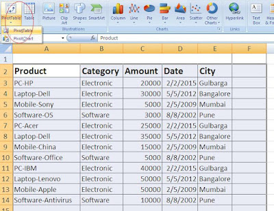
Step 2: Enter some data as following screen shot.

Step 3: Select your all data then click on "Insert" Tab and select "Pivot Table", follow below image.

Step 4: Select "range of data or cells" with sheet, follow the below screen.

Step 5: Drag the fields as per following screen shot to summarize your all data.

Step 6: Chart can be created without much effort, just click on "chart" and it will opens different chart type and select "Column" type[for this example only] and the chart is ready!. [refer below screen shot]

Advantages of Pivot table:-

1) A pivot table will quickly summarizes the data by any column, calculate average, sum, count, percentage etc.

2) Data can presented in a chart.

3) Data can grouped by year, category wise or date etc.

<<  Macro Example 

Creating an Excel form with Macros

This tutorial teaches you how to create an excel forms with Macros with step-by-step approaches. 

Step1 :  Open MS Excel Application and then click on “Developer” Tab  then click on “Visual Basic” option as shown in following screen shots. 

Step2: Click on “Insert” menu then select “UserForm” as shown in below image

Step3: Drag and drop the controls on the form (in this example:  3 Labels, 3 Text Boxes and 2 Buttons and set properties for Label1 to “Enter Product Name”, Label2 to “Enter Qty”, Label3 to “Enter Product Price”, Button1 to “AddNew Record” and Button2 to “Reset” in “Caption” under properties dialog box) follow below image.

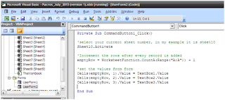
Step4: Now, Double click on “AddNew Record” button to write some code for inserting records to current sheet. Follow below screen image

Step 5: Now, test the form by running it, click on Green Forward arrow symbol or by pressing function key “F5” (see below image)

Step 6: You’ll see following output after pressing F5 or clicking on green forward arrow

Step 7: Enter a record as following and hit the “AddNew Record” Button. After this, one record is added to the sheet (sheet10 in this example)

Step8: Now close the form by clicking on “X” it will take you to the design mode. And enter some code for “Reset” button for resetting all values. Follow below image. [double click on “Reset” button and add following code]

Step9:  To call the User Form, which is created now, insert a button in the current sheet. [go to “Developer” tab and click -> Insert -> Command Button, drag on the sheet.   Follow below image.

Step 10: Right click on “ User Form” button and select “View Code”

Step 11: Enter following a line of code in it. Follow below image.

Step12: Now Click back on “Design Mode” to enable “User Form” button functioning, Click on “User Form” button and you’ll see following screen. [now start entering list of records] 

Step 13: Enter few more record by clicking on “AddNew Record” button and “Reset” for clearing all values.

That’s all for now! I’m coming with new Macro example in next blog.

Thank you!

Recording a Macro 

Pivot Table Demo